- Published on
Deutsch's Algorithm: One Query is Better Than Two Queries
- Authors

- Name
- Galih Laras Prakoso
- @galihlprakoso

This is another win for Quantum Computing over Classical Computing, to solve Deutsch's Problem, Quantum Computing needs less query compared to Classical Computing. What's Deutsch's Problem?
Deutsch's Problem
It's pretty simple, imagine a function , where . Your job is to simply determine whether the function is Constant or Balanced. What does it means? please look at this table:
0 | 0 | 0 | 0 |
1 | 0 | 1 | 1 |
0 | 1 | 0 | 1 |
1 | 0 | 1 | 1 |
We can divide these functions into two groups, constant: , , and balanced: , . In other way, we could see this problem as the same as doing to all possible outputs of given inputs :
0 | 0 | 0 |
0 | 1 | 1 |
1 | 0 | 1 |
1 | 1 | 0 |
As you can see that we could group the function by looking at their results of -ing all possible inputs .
Classical Computing
We can solve this problem using Classical Computing by querying all possible inputs to the function. Why two queries? Because, knowing doesn't give you enough information whether to determine whether it's a Constant or Balanced function. could still be 0 which will make this function Constant, or it could also be 1 which will make this function Balanced.
So, the best of what Classical Computing can do to solve this problem is by doing two queries.
Quantum Computing

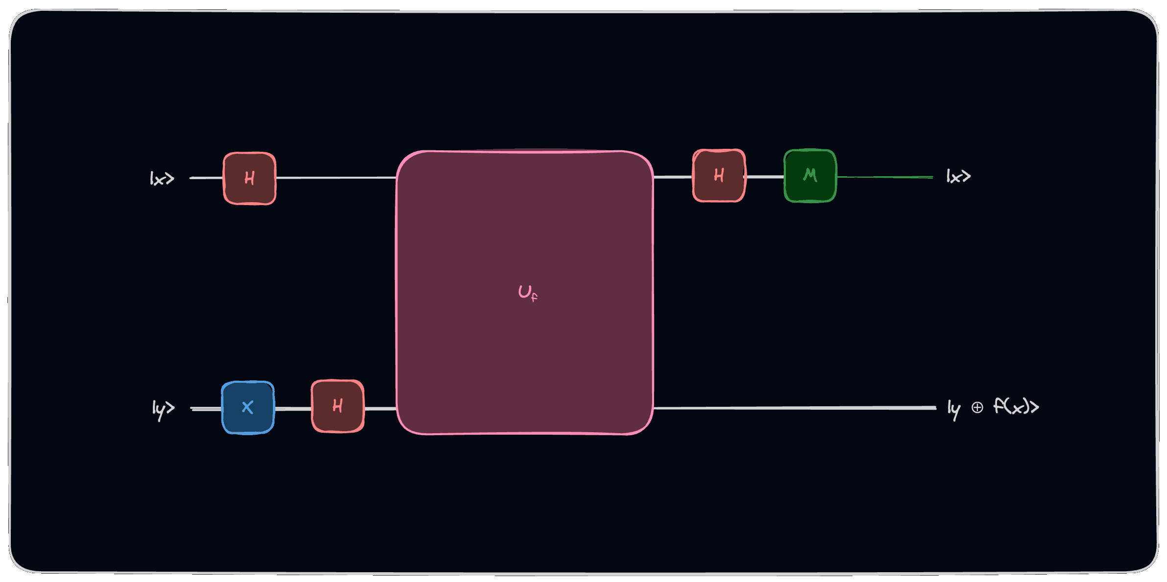
Better than Classical Computing, by using Quantum Computing, we're able to solve the Deutsch's Problem using just single query. All we need to have is a unitary matrix which is a permutation matrix that will somehow have the capability to the value of the first qubit with the second qubit .
As you can see that the circuit above is capable to solve the Deutsch's Problem by using just single query. By looking at the result of the measurement of the first qubit, we will be able to determine whether the function is Constant or Balance. It will output when the function is Constant and when the function is Balanced.
Mathematical Explanation
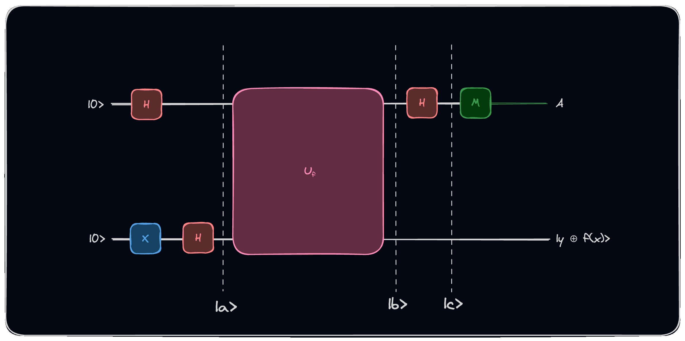
I will breakdown the explanation into three states, we will observe the evolution of the qubit states: ,,:

Initially we have this state:
We will keep the , because it will be easier to be used to explain the transformation to the next state after applying the gate:
Okay, it seems a little bit complicated 🙄, let's simplify the equation with one notes (we need to keep the state isolated), because it will intuitively tells us that the second qubit is unchanged. By observing the equation above, we could generalize the equation to be like this:
A gentle reminder: . By using this generalization, we could transform our state to be like this:
or
Actually, we can also take out :
When , we will get:
otherwise, when we will get:
Now, we arrived to the observation of last state . In this state, we just simply apply (Hadamard) operation to the first qubit and it will simply give us this states:
When , we will get:
When we will get:
As you can see that the second qubit is unchanged () while the first qubit's state is depending on the result of . After the measurement on the first qubit, we will get the classical value when the function is Constant and when the function is Balanced.
Qiskit Implementations
First, we need to define the four functions ,,,. All these four functions is just a quantum circuit with some qubit operations that represent the behaviour of each function:
Import qiskit library:
from qiskit import QuantumCircuit
: , :
def f_a() -> QuantumCircuit:
    circuit = QuantumCircuit(2)
    return circuit

print(f_a())
Output:
q_0:

q_1:
: , .
def f_b() -> QuantumCircuit:
    circuit = QuantumCircuit(2)
    circuit.cx(0, 1)
    return circuit

print(f_b())
Output:
q_0: ──■──
     ┌─┴─┐
q_1: ┤ X ├
     └───┘
: , .
def f_c() -> QuantumCircuit:
    circuit = QuantumCircuit(2)
    circuit.cx(0, 1)
    circuit.x(1)
    return circuit

print(f_c())
Output:
q_0: ──■───────
     ┌─┴─┐┌───┐
q_1: ┤ X ├┤ X ├
     └───┘└───┘
: , .
def f_d() -> QuantumCircuit:
    circuit = QuantumCircuit(2)
    circuit.x(1)
    return circuit

print(f_d())
Output:
q_0: ─────
     ┌───┐
q_1: ┤ X ├
     └───┘
Next, we need to create a circuit for our Deutsch Algorithm:
def deutsch_algo_circuit(function: QuantumCircuit):
    n = function.num_qubits - 1
    circuit = QuantumCircuit(n + 1, n)

    circuit.x(n)
    circuit.h(range(n + 1))

    circuit.barrier()
    circuit.compose(function, inplace=True)
    circuit.barrier()

    circuit.h(range(n))
    circuit.measure(range(n), range(n))

    return circuit

print(
    deutsch_algo_circuit(
        f_c()
    )
)
Output:
     ┌───┐      ░            ░ ┌───┐┌─┐
q_0: ┤ H ├──────░───■────────░─┤ H ├┤M├
     ├───┤┌───┐ ░ ┌─┴─┐┌───┐ ░ └───┘└╥┘
q_1: ┤ X ├┤ H ├─░─┤ X ├┤ X ├─░───────╫─
     └───┘└───┘ ░ └───┘└───┘ ░       ║
c: 1/════════════════════════════════╩═
                                     0
All we need to do now is just running our algorithm on Quantum Computing simulator:
from qiskit_aer import AerSimulator

circuit = deutsch_algo_circuit(f_c())
result = AerSimulator().run(circuit, shots=1, memory=True).result()
measurements = result.get_memory()

if measurements[0] == "0":
    print("constant")
else:
    print("balanced")
Output:
balanced
Yeay! We've successfully solve the Deutsch's Problem using Deutsch's Algorithm and run it on Quantum Computing simulator and get expected result. You could try to test another function and see whether it's returning the expected or not.
If you have anything to discuss, please drop your comments below! 🍻🍻